Solutions For Permanent Stationary Position Error
August 25, 2021
It looks like some users have encountered a steady state error code of constant position. There are a number of factors that can cause this problem. Now let’s talk about some of them.
Recommended: Fortect
Contents
Steady state error is probably defined as the difference between the input (command) portion and the system output at a time limit. goes, it becomes infinite (that is, when the answer has come to a steady state). The stationary error is likely to depend on the type of enclosing record. (Steps, ramps, etc.) as recordingssystem (0, I or II).
Note. The stationary failure research project is only useful for stable methods. You should always check the stability of the system first. Performing stationary fault analysis. Most of the methods we present will provide a solution even if the error persists. Don’t put yourself in the final stationary value.
Calculation Of Stationary Errors
Before discussing the relationship between stationary errors and system records, let’s show how errors are calculated independently. human body type or entrance. Then we will most likely begin to derive formulas that we can apply when the system has a different structure and Feedback is one of our standard measures. The stationary error can be calculated using the open or closed loop money transfer function. for bringing back Unity computers. For example, let’s say we are deploying the system below.
This is often equivalent to the following system, so t (s) isfeedback movement function.
We will most likely calculate the steady state error when using this system from a handoff or closed loop function using their final value. Course cost. Recall that this theorem is applicable only if the object of the new limit (in this case, sE (s)) already has negative poles with a real part.
Why not pass Laplace transforms to standard inputs and compute equations to compute errors in steady state calculations? as the open loop transfer function in each case.
Recommended: Fortect
Are you tired of your computer running slowly? Is it riddled with viruses and malware? Fear not, my friend, for Fortect is here to save the day! This powerful tool is designed to diagnose and repair all manner of Windows issues, while also boosting performance, optimizing memory, and keeping your PC running like new. So don't wait any longer - download Fortect today!

When we design a controller, we usually want to compensate for system failures as well. Let’s say we have the latest system with a malfunction that occurs as shown below.
This time, we can find the corresponding error for a sudden stationary disturbance by applying the final value theorem (process R (s) = 0).
If we have a unified feedback system, we have to be careful, because the incoming signal G (s) is no longer a real physical error E (s). Error The large difference between the set reference and the actual total output is E (s) = R (s) – Y (s). If the focus of the feedback is the walking function H (s), the signal subtracted from R (s) is no longer true Y (s), it is outputted as H (s). This situation can be illustrated below.
By manipulating the nature of the blocks, we can convert this system to return an equivalent allocation unit, as shown below.
System Type Followed By Permanent Error
If you refer to the equations for estimating stationary failures for systems of units, everyone will find that we have comments some specific constants (known as static error constants). They are always the same as the constant position (Kp), its velocity constant (Kv), and the acceleration and velocity constant (Ka). Knowing the value of this constant, as well as the type of the entire system, it is possible to predict whether our system will have a finite number.stationary failure.
First, we need to talk about the type of system. The system type is defined as the number of net integrators on the direct path Unified feedback system. That is, the exercise type is equal to the true value of n if the system is found to be represented in the next frame. It doesn’t matter if your integrators are part of the control or a factory.
Therefore, your system can be Type 8, Type 1, and so on. The following tables show how the stable error state changes depending on the course type.
| System Type 0 | Step by step | Ramp Entrance | Parabolic Entry |
|---|---|---|---|
| Steady State Error Formula | 1 / (1 + km) | 1 / qt | 1 / Ka |
| Static Error Constant | Kp = constant | Kv means 0 | Ka means 0 |
| Error | 1 / (1 + km) | endless | endless |
| Login | Step by step | Ramp Entrance | Parabolic Entry |
|---|---|---|---|
| Steady State Error Formula | 1 / (1 + km) | 1 / qt | 1 / Ka |
| Static Error Constant | Kp = infinite | Kv constant | Ka equals 0 |
| Error | 0 | 1 / qt | endless |
| Type 1 System | Step by step | Ramp Entrance | Parabolic Entry |
|---|---|---|---|
| Steady State Error Formula | 1 / (1 + km) | 1 / qt | 1 / Ka |
| Static Error Constant | Kp means infinity | Kv means infinity | Ka = constant |
| Error | 0 | 0 | 1 / Ka |
Example: Compliance With Inpatient Deficiency Treatment
In this example, let G (s) be equal to the following.
Since this system must be type 1, there are no stationary errors in step data and countless errors in parabolas. A source. The only record that results in the final stationary error in this particular system a is the ramp record. We want to choose K so that the closed-loop system has a steady state of 0.1, which is very error-prone with respect to the ramp setting. criticize those first Ramp return input for amplification K 0 =.
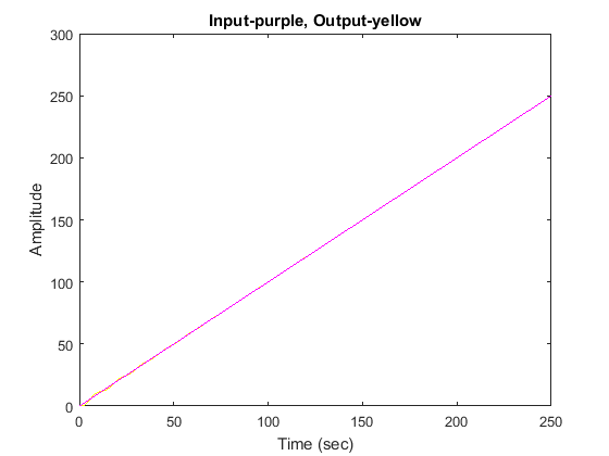
s = tf ('s');G = ((s + 3) * (s + 5)) / (s * (s + 7) * (s + 8));T implies feedback (G, 1);t = 0: 0.1: 25;u = equal to t;[y, t, x] lsim (T, u, t);plot (t, y, 'y', t, u, 'm')xlabel ('time (sec.)')ylabel ('Amplitude')title ('purple, yellow')The steady-state error in this system is quite large, given that the output in 20 seconds was approximately 16 versus actual input 20 (steady-state error may be about 4). Let’s take a closer look at this.
From our definition of the problem, we understood that stationary The error should often be 0.1. Thus, we can solve the following problems. these steps:
Let’s see that the input ramp response for K is 37.33 by entering the following law in the MATLAB command window. matches

Download this software and fix your PC in minutes.
Steady state error is defined as the ratio between the input (control) and the output of the system, usually at the limit when time is infinite (that is, when the response has reached a steady state). Stationary error can also depend on the type of understanding (step, tilt, etc.), as well as the type of system (0, I, or possibly II).
The system positional error constant is determined for a completely new step record. Systems with this finite stationary error with an unequal zero with respect to first order polynomial wisdom (ramp input) are called Type 1 systems. The velocity error constant for the device is specified for the slope input.